SQL Normalization and Denormalization: The Performance Mirror

In the beginning, we are taught to normalize. "Repeat nothing," the professors say. This is the law of Transactional Integrity (OLTP). But when you build a dashboard that calculates real-time revenue across 10 million orders, and your "Perfectly Normalized" query takes 5 seconds because of a 15-way JOIN, the math fails the reality of the user experience.

As an Architect, you don't choose one or the other. You build a Performance Mirror.

---

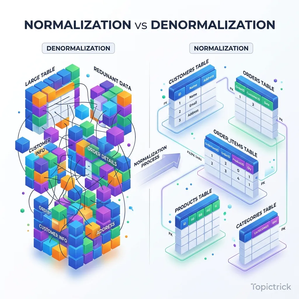
1. Normalization: The Mathematical Rigor

Normalization is the process of organizing data to minimize redundancy and prevent anomalies. It is the "Physical Jail" for your data to ensure it never gets corrupted.

1.1 The Physics of Data Alignment: 1NF and Byte-Padding

Many developers think "1st Normal Form" is just about "No repeating groups." But at the hardware level, it's about Predictable Offsets.

• The Physics: If a row has a variable number of columns or "List" types, the database engine cannot know exactly where on the disk a specific field starts. It has to "Scan and Parse" every row.
• The Mirror: By enforcing 1NF, every column has a fixed type (or a pointer to a toast table). This allows the CPU to calculate the exact Memory Offset of a field.
• The Byte Reality: Modern databases like Postgres perform Data Alignment. If you have a char(1) followed by an int4, the database adds 3 bytes of "Padding" to ensure the integer starts on a 4-byte boundary. A perfectly normalized schema with optimized column order (largest types first) can reduce your storage footprint by 15% without deleting a single bit of data.

---

2. The Cost of Perfection: The Join Geometry

Every time you normalize, you create a Join Requirement. To see a user's address, the engine must:

1. Find the user in the users table.
2. Get the address_id.
3. Jump to the addresses table (Random I/O).
4. Match the keys.

The CPU Penalty

JOINs are the most expensive operations in SQL. The database must use algorithms like Nested Loops, Hash Joins, or Merge Joins to stitch the data back together.

• The L1/L2 Cache Locality Mirror: In a normalized database, the data you need is spread across different physical pages on the SSD. The CPU cannot "pre-fetch" the address data while it's reading the user data. This "Cache Miss" is the physical reason why JOIN-heavy queries are slow.

---

3. Denormalization: The Hardware-Mirror Trick

Denormalization is the intentional introduction of redundancy to speed up reads. You are "Spending" disk space to "Save" CPU time.

3.1 Architecting the Materialized Denormalization Mirror

Beyond simple "Redundant Columns," we use Materialized Denormalization.

• The Concept: Instead of your app calculating a "Summary" on every request, you maintain a Derived Table.
• The Sync Mirror: This isn't just a copy; it's a Functional Mirror. You use Logical Replication or CDC (Change Data Capture) to stream updates from your 3NF master to your denormalized mirrors.
• The Win: Your transactional database stays "Pure" and small (high cache hit ratio), while your "Search Mirror" is flat, redundant, and optimized for sub-millisecond full-text scans.

---

4. The Hybrid Mirror: Materialized Redundancy

How do you get the Integrity of 3NF with the Speed of Denormalization?

Pattern 1: Triggers for Aggregates

Instead of running SUM(price) every time a user looks at their cart, you add a total_price column to the carts table.

• The Sync: You use a Database Trigger to update the total_price every time an item is added.
• The Tradeoff: You have made the INSERT slower (Write Amplification) to make the SELECT instant.

Pattern 2: Materialized Views

As explored in Module 20, Materialized Views are the "Ultimate Denormalization." You keep your source of truth perfectly normalized in 3NF, but you tell the database to "Calculate and cache" a denormalized version for the API.

---

5. Case Study: The "Social Feed" Architecture

5.1 Case Study: When 3NF kills a Real-Time Dashboard

A global SaaS provider built their "Billing Dashboard" on a perfectly normalized 3NF schema. To show the "Unpaid Balance" for a client, the query had to join Clients -> Invoices -> LineItems -> Payments.

• The Problem: With 50 million line items, the dashboard took 12 seconds to load. The "Join Complexity" caused the database to spill the Join Buffer to the SSD.
• The Denormalized Fix: They added a current_unpaid_balance column to the Clients table and updated it via a trigger on the Invoices table.
• The Result: The 12-second dashboard load became 4 milliseconds. They traded the risk of a small inconsistency (fixable via a nightly reconciliation cron) for a massive increase in customer satisfaction.

---

6. Summary: The Architecture Checklist

1. 3NF for OLTP: Use strict normalization for core entities to prevent data corruption.
2. Byte Alignment: Order your columns from largest to smallest to avoid wasted "Padding" bytes in the physical row.
3. Denormalize for "Hot" Paths: If a query has 5+ JOINS and high frequency, add redundant columns.
4. The CDC Mirror: Use Change Data Capture for complex denormalization mirrors to avoid blocking transactions with heavy triggers.
5. Audit the Debt: Run a monthly check for "Data Drift" (inconsistencies) in your denormalized tables.

Database design is the "Soil" in which your application grows. By mastering the balance between the mathematical purity of Normalization and the hardware-driven speed of Denormalization, you gain the power to build systems that are both Indestructible and Lightning Fast. You graduate from "Following rules" to "Engineering Tradeoffs."

---

Phase 23: Normalization Mastery Action Items

• Identify one query with 4+ joins and analyze its Join Buffer usage.
• Optimize column order in your largest table to minimize bit-padding waste.
• Add a "Redundant" aggregate column to eliminate a heavy SUM() join.
• Advanced Goal: Implement a CDC-based Denormalization Mirror for a high-traffic reporting endpoint.

Read next: SQL Performance Tuning: Mastery of EXPLAIN ANALYZE →

Frequently Asked Questions

Q: What is the difference between normalisation and denormalisation?

Normalisation reduces redundancy by splitting data into multiple related tables — each fact is stored once, updates propagate correctly, and storage is minimised. Denormalisation intentionally reintroduces redundancy — duplicating data across tables or adding pre-computed columns — to improve read query performance by reducing joins. Normalise for data integrity and write correctness; denormalise for read speed when measured query performance demands it. Most transactional databases use normalised schemas; reporting and analytics databases (data warehouses) use heavily denormalised star or snowflake schemas.

Q: What is a star schema and when is it used?

A star schema organises data around a central fact table containing numeric measurements (sales amount, quantity) surrounded by dimension tables containing descriptive attributes (product, customer, date, store). It is called a star because the ERD looks like a star. Star schemas are used in data warehouses and BI tools because they are simple to query (few joins needed), intuitive for business users, and optimised for columnar storage and aggregation. Analytical queries like "total revenue by product category by month" run efficiently against a star schema, while they would require complex joins in a fully normalised OLTP schema.

Q: What is the difference between an OLTP and an OLAP database schema?

OLTP (Online Transaction Processing) schemas are highly normalised — they optimise for fast individual row lookups, inserts, and updates with minimal redundancy. They support the operational systems (e-commerce transactions, banking records, inventory updates). OLAP (Online Analytical Processing) schemas are denormalised — they optimise for aggregating large volumes of data across many rows and columns for reporting and analytics. Running analytical queries on an OLTP schema causes full table scans that degrade operational performance; running transactional workloads on an OLAP schema causes write amplification. Mature architectures separate the two, using ETL pipelines to move OLTP data into an OLAP store.

Part of the SQL Mastery Course — engineering the balance.