Vector Database Optimisation: Chunking & Scaling

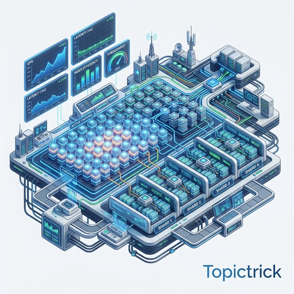
Vector Database Production Optimisation: The Key Techniques

The most impactful optimisations for a production vector database are, in order: semantic chunking strategy (the single biggest factor in retrieval quality), embedding model selection matched to your query type, HNSW index tuning (especially search_ef, which defaults to 10 in ChromaDB but should be 50–100), two-stage retrieval with cross-encoder re-ranking, hybrid search combining vector and keyword, Redis query caching, and monitoring for zero-result and low-similarity rates.

A vector database that works well in a demo often behaves completely differently in production. You added 1,000 chunks during development. In production you have 500,000 — and queries that took 20 ms now take 800 ms. Your RAG pipeline was returning great answers in testing. In production, users complain the answers feel generic. You think it is the LLM. It is actually the retrieval.

This post covers the techniques that separate a demo-grade vector search system from a production-grade one: advanced chunking strategies, embedding model selection, HNSW index tuning, hybrid search, query caching, monitoring, and scaling patterns.

This is the advanced post in the series. You should already be comfortable with the basics from the earlier posts: What is a Vector Database?, ChromaDB Tutorial, and Build a Semantic Search Engine from Scratch.

1. Chunking Strategy — The Most Impactful Decision

The single biggest factor in retrieval quality is not your vector database or your embedding model — it is how you chunk your documents. Poor chunking causes your system to retrieve irrelevant or incomplete context regardless of how good everything else is.

Fixed-Size Chunking (Baseline)

Split by character count with overlap. Simple, predictable, and good enough for many use cases.

python

def fixed_size_chunks(text: str, size: int = 500, overlap: int = 100) -> list[str]:
    chunks = []
    step = size - overlap
    for start in range(0, len(text), step):
        chunk = text[start:start + size].strip()
        if chunk:
            chunks.append(chunk)
    return chunks

Problem: A 500-character boundary might land in the middle of a sentence or split a code example in half. The resulting chunk loses semantic coherence.

Sentence-Aware Chunking (Better)

Use NLTK or spaCy to split at sentence boundaries, then group sentences into target-sized chunks:

python

import nltk
nltk.download("punkt_tab", quiet=True)

def sentence_chunks(text: str, max_chars: int = 600, overlap_sentences: int = 1) -> list[str]:
    sentences = nltk.sent_tokenize(text)
    chunks = []
    current = []
    current_len = 0

    for sentence in sentences:
        sentence_len = len(sentence)
        if current_len + sentence_len > max_chars and current:
            chunks.append(" ".join(current))
            # Overlap: keep last N sentences for next chunk
            current = current[-overlap_sentences:] if overlap_sentences else []
            current_len = sum(len(s) for s in current)
        current.append(sentence)
        current_len += sentence_len

    if current:
        chunks.append(" ".join(current))

    return chunks

This respects sentence boundaries, dramatically improving chunk coherence.

Semantic Chunking (Best for Long Documents)

Split based on topic shifts — when the semantic similarity between consecutive sentences drops below a threshold, start a new chunk. This keeps topically coherent content together.

python

from sentence_transformers import SentenceTransformer
import numpy as np

def semantic_chunks(
    text: str,
    model: SentenceTransformer,
    similarity_threshold: float = 0.75,
    max_chunk_chars: int = 1000,
) -> list[str]:
    """
    Split text at points where topic changes (cosine similarity < threshold).
    Falls back to character limit if no natural break is found.
    """
    sentences = nltk.sent_tokenize(text)
    if len(sentences) <= 2:
        return [text]

    embeddings = model.encode(sentences, batch_size=32, show_progress_bar=False)

    # Compute similarity between consecutive sentences
    similarities = [
        float(np.dot(embeddings[i], embeddings[i + 1]) /
              (np.linalg.norm(embeddings[i]) * np.linalg.norm(embeddings[i + 1])))
        for i in range(len(embeddings) - 1)
    ]

    # Split at topic boundaries
    chunks = []
    current = [sentences[0]]
    current_len = len(sentences[0])

    for i, (sentence, sim) in enumerate(zip(sentences[1:], similarities)):
        topic_break = sim < similarity_threshold
        too_long = current_len + len(sentence) > max_chunk_chars

        if topic_break or too_long:
            if current:
                chunks.append(" ".join(current))
            current = [sentence]
            current_len = len(sentence)
        else:
            current.append(sentence)
            current_len += len(sentence)

    if current:
        chunks.append(" ".join(current))

    return chunks

Which Chunking Strategy to Use

Fixed-size: fastest, adequate for homogeneous content. Sentence-aware: best balance of quality and speed for most RAG applications. Semantic chunking: highest quality for long mixed-topic documents (e.g., legal contracts, research papers) — but the extra embedding pass doubles ingestion cost.

2. Embedding Model Selection

Not all embedding models produce equally useful vectors for your task. The wrong model can degrade retrieval quality by 20–40%.

Matching Model to Task

Task	Recommended Model	Dimensions
General semantic search	`all-MiniLM-L6-v2`	384
High accuracy semantic search	`all-mpnet-base-v2`	768
Question → document retrieval	`multi-qa-MiniLM-L6-cos-v1`	384
Code search	`krlvi/sentence-msmarco-bert-base-dot-v5`	768
Multilingual	`paraphrase-multilingual-MiniLM-L12-v2`	384
Highest quality (paid)	`text-embedding-3-large` (OpenAI)	3072

For RAG applications — where you embed queries and retrieve document chunks — use a model designed for asymmetric retrieval (short question → long document). multi-qa-MiniLM-L6-cos-v1 and multi-qa-mpnet-base-dot-v1 are specifically trained for this.

Benchmarking Your Embedding Model

Never assume a model will work well for your domain. Build a small evaluation set and measure retrieval quality:

python

from sentence_transformers import SentenceTransformer
import numpy as np

def evaluate_retrieval(model_name: str, test_cases: list[dict]) -> dict:
    """
    Evaluate retrieval quality.
    test_cases: list of {'query': str, 'relevant_doc': str, 'all_docs': list[str]}
    Returns hit@1, hit@3, mean_rank metrics.
    """
    model = SentenceTransformer(model_name)
    hits_at_1 = 0
    hits_at_3 = 0
    ranks = []

    for case in test_cases:
        all_docs = case["all_docs"]
        doc_embeddings = model.encode(all_docs, normalize_embeddings=True)
        query_embedding = model.encode(case["query"], normalize_embeddings=True)

        scores = np.dot(doc_embeddings, query_embedding)
        ranked_indices = np.argsort(scores)[::-1]

        relevant_idx = all_docs.index(case["relevant_doc"])
        rank = list(ranked_indices).index(relevant_idx) + 1
        ranks.append(rank)

        if rank == 1:
            hits_at_1 += 1
        if rank <= 3:
            hits_at_3 += 1

    n = len(test_cases)
    return {
        "model": model_name,
        "hit@1": hits_at_1 / n,
        "hit@3": hits_at_3 / n,
        "mean_rank": sum(ranks) / n,
    }


# Compare two models on your domain
test_cases = [
    {
        "query": "how to reset password",
        "relevant_doc": "Go to Account Settings and click Reset Password to change your credentials.",
        "all_docs": [
            "Go to Account Settings and click Reset Password to change your credentials.",
            "Invoice history is available in the billing section of your account.",
            "Contact support if your device fails to start after the update.",
        ]
    },
    # ... add more test cases
]

for model in ["all-MiniLM-L6-v2", "multi-qa-MiniLM-L6-cos-v1"]:
    print(evaluate_retrieval(model, test_cases))

Building even 20–30 test cases and running this evaluation before committing to a model can save hours of debugging poor retrieval later.

3. HNSW Index Tuning

HNSW (Hierarchical Navigable Small World) is the index algorithm used by ChromaDB, Qdrant, and Weaviate. Three parameters control the quality/speed trade-off:

M — number of bi-directional links per node. Higher M improves recall but increases memory and indexing time. Default: 16. For high-recall applications: 32–64.

ef_construction — the size of the dynamic candidate list during index build. Higher values improve recall but slow down ingestion. Default: 100. For high-recall: 200–400.

ef_search (or hnsw:search_ef in ChromaDB) — the candidate list size at query time. Higher values improve recall and slow queries. This is the most useful runtime trade-off parameter.

python

# ChromaDB HNSW tuning
collection = client.get_or_create_collection(
    name="production_docs",
    metadata={
        "hnsw:space": "cosine",
        "hnsw:M": 32,                  # double the default for better recall
        "hnsw:construction_ef": 200,   # better index quality
        "hnsw:search_ef": 100,         # better query recall (default: 10 — far too low)
    }
)

ChromaDB Default search_ef is 10

ChromaDB's default hnsw:search_ef is 10, which is very conservative. For production RAG applications, set it to at least 50–100. A search_ef of 10 on a large collection can miss highly relevant results and is the most common cause of poor retrieval quality in ChromaDB deployments.

pgvector HNSW tuning:

sql

-- Set ef_search at query time (per session or globally)
SET hnsw.ef_search = 100;

-- Or set a higher default in the index
CREATE INDEX ON documents
USING hnsw (embedding vector_cosine_ops)
WITH (m = 32, ef_construction = 200);

4. Hybrid Search: Combining Vector and Keyword

Pure vector search is excellent for semantic queries but can miss exact matches that keyword search would catch trivially (product codes, technical identifiers, proper nouns). Hybrid search combines both.

Hybrid Search with pgvector + Full-Text Search

Postgres has native full-text search (tsvector). Combine it with pgvector in a single query using Reciprocal Rank Fusion (RRF):

sql

-- Add full-text search column
ALTER TABLE documents ADD COLUMN fts_vector tsvector
    GENERATED ALWAYS AS (to_tsvector('english', content)) STORED;
CREATE INDEX ON documents USING gin(fts_vector);

-- Hybrid query using RRF scoring
WITH semantic AS (
    SELECT id, 1 - (embedding <=> %(query_vector)s::vector) AS score,
           ROW_NUMBER() OVER (ORDER BY embedding <=> %(query_vector)s::vector) AS rank
    FROM documents
    LIMIT 20
),
keyword AS (
    SELECT id,
           ts_rank(fts_vector, plainto_tsquery('english', %(query_text)s)) AS score,
           ROW_NUMBER() OVER (
               ORDER BY ts_rank(fts_vector, plainto_tsquery('english', %(query_text)s)) DESC
           ) AS rank
    FROM documents
    WHERE fts_vector @@ plainto_tsquery('english', %(query_text)s)
    LIMIT 20
),
rrf AS (
    SELECT
        COALESCE(s.id, k.id) AS id,
        COALESCE(1.0 / (60 + s.rank), 0) + COALESCE(1.0 / (60 + k.rank), 0) AS rrf_score
    FROM semantic s
    FULL JOIN keyword k ON s.id = k.id
)
SELECT d.id, d.content, r.rrf_score
FROM rrf r
JOIN documents d ON d.id = r.id
ORDER BY r.rrf_score DESC
LIMIT 5;

Reciprocal Rank Fusion (the 1.0 / (60 + rank) formula) normalises scores from different systems into a comparable range and combines them without needing to calibrate weights. The constant 60 dampens the impact of very high ranks.

Hybrid Search with ChromaDB (Manual)

ChromaDB does not have built-in keyword search, but you can implement hybrid search manually:

python

from rank_bm25 import BM25Okapi   # pip install rank-bm25
import numpy as np

class HybridSearchEngine:
    def __init__(self, collection, documents: list[str]):
        self.collection = collection
        self.documents = documents
        # Build BM25 index
        tokenised = [doc.lower().split() for doc in documents]
        self.bm25 = BM25Okapi(tokenised)

    def search(self, query: str, n_results: int = 5, alpha: float = 0.5) -> list[dict]:
        """
        alpha: weight of semantic score (1-alpha = keyword weight)
        """
        # Vector search
        vector_results = self.collection.query(
            query_texts=[query], n_results=n_results * 2,
            include=["documents", "distances", "metadatas"]
        )
        vector_scores = {
            doc: 1 - dist
            for doc, dist in zip(
                vector_results["documents"][0],
                vector_results["distances"][0]
            )
        }

        # BM25 keyword search
        bm25_scores = self.bm25.get_scores(query.lower().split())
        max_bm25 = max(bm25_scores) if max(bm25_scores) > 0 else 1
        bm25_normalised = {
            self.documents[i]: score / max_bm25
            for i, score in enumerate(bm25_scores)
            if score > 0
        }

        # Combine with RRF-style weighting
        all_docs = set(vector_scores.keys()) | set(bm25_normalised.keys())
        combined = []
        for doc in all_docs:
            v_score = vector_scores.get(doc, 0)
            k_score = bm25_normalised.get(doc, 0)
            combined_score = alpha * v_score + (1 - alpha) * k_score
            combined.append({"text": doc, "score": combined_score})

        combined.sort(key=lambda x: x["score"], reverse=True)
        return combined[:n_results]

5. Query Caching

Identical or near-identical queries are common in production (users asking the same FAQ questions repeatedly). Cache results to avoid redundant embedding and retrieval operations.

python

import hashlib
import json
from functools import lru_cache
from datetime import datetime, timedelta

class CachedSearchEngine:
    def __init__(self, engine, cache_ttl_seconds: int = 300):
        self.engine = engine
        self.cache: dict[str, tuple[list, datetime]] = {}
        self.ttl = timedelta(seconds=cache_ttl_seconds)

    def _cache_key(self, query: str, n_results: int, filters: dict | None) -> str:
        payload = {"q": query.lower().strip(), "n": n_results, "f": filters or {}}
        return hashlib.md5(json.dumps(payload, sort_keys=True).encode()).hexdigest()

    def search(self, query: str, n_results: int = 5, filters: dict | None = None) -> list[dict]:
        key = self._cache_key(query, n_results, filters)
        now = datetime.utcnow()

        if key in self.cache:
            results, cached_at = self.cache[key]
            if now - cached_at < self.ttl:
                return results   # cache hit

        results = self.engine.search(query, n_results=n_results, filters=filters)
        self.cache[key] = (results, now)
        return results

    def invalidate(self) -> None:
        """Clear the entire cache (e.g., after re-ingestion)."""
        self.cache.clear()

For production at scale, replace the in-memory dict with Redis:

python

import redis
import json

redis_client = redis.Redis(host="localhost", port=6379, decode_responses=True)

def cached_search(engine, query: str, n_results: int = 5, ttl: int = 300) -> list[dict]:
    cache_key = f"search:{hashlib.md5(f'{query}:{n_results}'.encode()).hexdigest()}"
    cached = redis_client.get(cache_key)
    if cached:
        return json.loads(cached)

    results = engine.search(query, n_results=n_results)
    redis_client.setex(cache_key, ttl, json.dumps(results))
    return results

6. Re-ranking Results

Vector search returns the top-K most similar chunks, but similarity to the query vector is not always the best measure of relevance. A re-ranker (cross-encoder model) takes the query and each candidate chunk as a pair and produces a more accurate relevance score.

python

from sentence_transformers import CrossEncoder

# Cross-encoders are slower but much more accurate than bi-encoders for ranking
reranker = CrossEncoder("cross-encoder/ms-marco-MiniLM-L-6-v2")

def retrieve_and_rerank(
    collection,
    query: str,
    initial_n: int = 20,
    final_n: int = 5
) -> list[dict]:
    """
    Two-stage retrieval:
    1. Fast ANN search to get top-20 candidates
    2. Accurate cross-encoder re-ranking to select top-5
    """
    # Stage 1: fast vector retrieval (over-retrieve)
    results = collection.query(
        query_texts=[query],
        n_results=initial_n,
        include=["documents", "metadatas"]
    )
    candidates = results["documents"][0]
    metas = results["metadatas"][0]

    # Stage 2: cross-encoder re-ranking
    pairs = [(query, doc) for doc in candidates]
    rerank_scores = reranker.predict(pairs)

    ranked = sorted(
        zip(candidates, rerank_scores, metas),
        key=lambda x: x[1],
        reverse=True
    )

    return [
        {"text": doc, "rerank_score": float(score), "metadata": meta}
        for doc, score, meta in ranked[:final_n]
    ]

Re-ranking adds 50–200 ms of latency but can dramatically improve retrieval quality, especially for complex queries. It is the technique used by Cohere Rerank, Pinecone's rerank API, and Voyage AI.

7. Monitoring and Observability

You cannot optimise what you cannot measure. Track these metrics in production:

python

import time
from dataclasses import dataclass, field
from collections import defaultdict

@dataclass
class SearchMetrics:
    total_queries: int = 0
    cache_hits: int = 0
    latencies_ms: list[float] = field(default_factory=list)
    zero_result_queries: list[str] = field(default_factory=list)
    low_similarity_queries: list[str] = field(default_factory=list)

    def record_query(
        self,
        query: str,
        latency_ms: float,
        results: list[dict],
        cache_hit: bool,
        low_similarity_threshold: float = 0.4
    ) -> None:
        self.total_queries += 1
        self.latencies_ms.append(latency_ms)
        if cache_hit:
            self.cache_hits += 1
        if not results:
            self.zero_result_queries.append(query)
        elif results[0]["similarity"] < low_similarity_threshold:
            self.low_similarity_queries.append(query)

    def report(self) -> dict:
        lats = self.latencies_ms
        return {
            "total_queries": self.total_queries,
            "cache_hit_rate": self.cache_hits / max(self.total_queries, 1),
            "p50_latency_ms": sorted(lats)[len(lats) // 2] if lats else 0,
            "p95_latency_ms": sorted(lats)[int(len(lats) * 0.95)] if lats else 0,
            "zero_result_rate": len(self.zero_result_queries) / max(self.total_queries, 1),
            "low_similarity_rate": len(self.low_similarity_queries) / max(self.total_queries, 1),
            "recent_zero_result_queries": self.zero_result_queries[-10:],
            "recent_low_similarity_queries": self.low_similarity_queries[-10:],
        }

Key metrics to alert on:

p95 query latency > 500 ms: signals HNSW tuning or hardware is needed
Zero-result rate > 5%: suggests gaps in your document corpus
Low similarity rate > 20%: suggests chunking, embedding model, or corpus coverage issues
Cache hit rate < 10%: high query diversity — caching may not help much, focus on index tuning

8. Scaling Patterns

When ChromaDB Starts Slowing Down

ChromaDB runs on a single machine. When queries start taking more than 200 ms at your target collection size, consider:

Tune HNSW first — increase hnsw:M and hnsw:construction_ef before re-indexing
Add a Redis cache for repeated queries
Partition by metadata — split one large collection into multiple smaller ones by category or date range, and route queries to the appropriate partition
Migrate to Qdrant or pgvector when the single-machine ceiling is reached

Migrating from ChromaDB to Qdrant

python

from qdrant_client import QdrantClient
from qdrant_client.models import Distance, VectorParams, PointStruct

qdrant = QdrantClient(host="localhost", port=6333)

# Create Qdrant collection
qdrant.create_collection(
    collection_name="production_docs",
    vectors_config=VectorParams(size=384, distance=Distance.COSINE),
)

# Export from ChromaDB
all_data = chroma_collection.get(include=["embeddings", "documents", "metadatas"])

# Import to Qdrant in batches
batch_size = 1000
points = [
    PointStruct(
        id=i,
        vector=embedding,
        payload={"text": doc, **meta}
    )
    for i, (embedding, doc, meta) in enumerate(zip(
        all_data["embeddings"],
        all_data["documents"],
        all_data["metadatas"]
    ))
]

for i in range(0, len(points), batch_size):
    qdrant.upsert(
        collection_name="production_docs",
        points=points[i:i + batch_size]
    )

print(f"Migrated {len(points)} vectors to Qdrant")

Production Optimisation Checklist

☐ Use sentence-aware or semantic chunking instead of naive fixed-size splits
☐ Benchmark your embedding model on a domain-specific evaluation set before committing
☐ Set hnsw:search_ef to at least 50–100 in ChromaDB (default of 10 is too low)
☐ Over-retrieve (top-20) then re-rank (select top-5) for high-quality RAG applications
☐ Add Redis-backed query caching for common/repeated queries
☐ Implement hybrid search (vector + BM25/FTS) if your corpus contains exact-match-critical content
☐ Monitor p95 query latency, zero-result rate, and low-similarity rate
☐ Review low-similarity queries weekly to identify corpus gaps
☐ Plan migration to Qdrant or Pinecone before you hit ChromaDB's single-machine ceiling

Key Takeaways

Chunking strategy is the highest-impact optimisation — sentence-aware or semantic chunking consistently outperforms fixed-size splits
Embedding model selection matters — use asymmetric retrieval models for question-to-document RAG
ChromaDB's default search_ef = 10 is the most common source of poor recall in production — set it to 50–100
Two-stage retrieval (ANN + cross-encoder re-ranking) gives the best quality at acceptable latency
Hybrid search (vectors + keyword) handles both semantic and exact-match queries correctly
Monitor the metrics that matter: zero-result rate and low-similarity rate tell you about corpus quality; p95 latency tells you about infrastructure

Vector Database Series — Complete

You have now completed the full Vector Database Series:

What is a Vector Database? The Complete Beginner's Guide
ChromaDB Tutorial: The Complete Beginner's Guide
ChromaDB vs Pinecone vs pgvector: Which Should You Use?
Build a Semantic Search Engine from Scratch
Vector Database Optimisation for Production ← you are here

For the next natural step — connect your vector database to an LLM and build a complete RAG pipeline — see Project: Build a RAG App with Claude.

For primary documentation on the tools used in this post: ChromaDB HNSW configuration reference, Pinecone performance optimisation guide, and the pgvector HNSW indexing documentation. Related posts in this series: What is a Vector Database? and ChromaDB vs Pinecone vs pgvector.

External references: